Queueing Theory for SREs: Little's Law and the Utilisation Knee

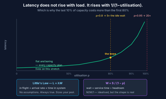
Nothing changed. Traffic went up 12%. p99 went up 400%. This curve is why.

Every SRE meets this situation eventually. The service has been fine for months. Traffic grows gradually. CPU is at 75% and nobody is worried, because 75% is not 100%. Then over two weeks p99 latency goes from 120ms to 900ms, and nothing in the code changed.

The instinct is to look for a regression — a slow query, a leak, a bad deploy. There is no regression. The system is doing exactly what queueing theory says it will do, and it would have been predictable weeks earlier by anyone who knew to look for the curve.

You do not need the field. You need two formulas.

Little’s Law: L = λW

The average number of items in a stable system equals the arrival rate times the average time each spends in it.

L = λ × W

L = items in the system (in flight, including queued)
λ = arrival rate (requests per second)
W = time in the system (seconds)

What makes this remarkable is what it does not assume. No assumption about the arrival distribution, the service time distribution, or the queue discipline. It holds for any stable system where things go in and come out. That generality is why it is the most practically useful result in the field.

It sizes pools. You handle 500 requests/second, each taking 200ms:

L = 500 × 0.2 = 100 concurrent requests

You need 100 workers to keep up. Ninety and the queue grows without bound. This is the calculation behind every thread pool, connection pool, and worker count in your system — whether or not anyone did it explicitly.

It runs in reverse to find hidden waiting. You measure 50 in-flight requests at 100 requests/second:

W = L / λ = 50 / 100 = 500ms

If your service time is 50ms, then 450ms of every request is spent waiting, not working. No profiler will show you that, because nothing is executing during it. This single computation has located more latency problems than most profiling sessions.

It is the fastest way to spot the doomed queue. A queue 10,000 deep draining at 500/second is imposing 20 seconds of delay. If callers time out at 2 seconds, every item in that queue is already worthless. The system is at 100% utilisation producing nothing — which is precisely the state a bounded queue exists to prevent.

The knee: W = S / (1 − ρ)

The second formula is the one that explains the cliff. For a simple single-server queue with random arrivals — the M/M/1 model — the time in system is:

W = S / (1 − ρ)

S = service time (how long the work takes when nothing is in the way)
ρ = utilisation (0 to 1)

Put numbers in it and the shape is immediately obvious:

Utilisation	Multiplier on service time	100ms of work takes
10%	1.1×	111ms
50%	2×	200ms
70%	3.3×	333ms
80%	5×	500ms
90%	10×	1,000ms
95%	20×	2,000ms
99%	100×	10,000ms

Latency is not a function of load. It is a function of remaining headroom. As ρ approaches 1, 1 − ρ approaches zero, and the quotient goes to infinity. The curve is flat and boring up to roughly 70%, then goes near-vertical.

Three consequences that change how you work:

Going from 70% to 80% utilisation costs you 50% more latency. Going from 90% to 95% doubles it again. The last slice of capacity is enormously more expensive than the first, measured in latency rather than in dollars.

Your traffic growth chart is a lie about what is coming. Traffic is linear on the dashboard. Latency is hyperbolic in utilisation. The two weeks in which nothing seemed to be happening were the flat part of the curve, and there is no gradual warning before the steep part.

Free CPU is not idle CPU; it is your latency budget. When someone asks why you run at 65% and proposes consolidating for cost savings, this is the answer, and it is quantitative: the 35% headroom is what is keeping p99 at 200ms instead of 1,000ms. That reframes a capacity argument from “engineers being cautious” into a priced trade-off, which is the only form in which it gets taken seriously.

M/M/1 is an idealisation — real services have multiple servers, non-random arrivals, and non-exponential service times, and the exact numbers will differ. The shape does not. Every queueing model has the 1/(1−ρ) term, because it comes from the structure of queueing rather than from the distributions.

Variability is the third dimension

Utilisation is not the whole story. Two systems at 70% can behave completely differently depending on how variable they are.

Kingman’s approximation makes the relationship explicit:

W ≈ (ρ / (1 − ρ)) × ((c²ₐ + c²ₛ) / 2) × S
             ↑              ↑
        utilisation    variability

c²ₐ and c²ₛ are the squared coefficients of variation for arrivals and service times. The important reading: waiting time is the product of a utilisation term and a variability term, so halving variability reduces waiting exactly as much as reducing utilisation by the equivalent amount.

The reason variability hurts is worth internalising because it is not intuitive: a queue cannot bank idle time. A burst that arrives while the server is busy creates a wait, and the idle period that follows does not refund it. Averages are preserved; the waiting is not.

This turns several things you already do into capacity work:

• Smoothing traffic is capacity. Jittered cron schedules, staggered client polling, and rate limiting at the edge all reduce c²ₐ. A fleet of clients all polling on the minute is a self-inflicted variability problem, and jitter fixes it for free.
• Tightening the service-time distribution is capacity. Cutting p99 service time without touching the mean reduces c²ₛ and therefore reduces queueing for everything, including the fast requests. This is why one slow endpoint degrades an entire service — it is not stealing CPU so much as inflating the variability term for every request sharing the pool.
• Separating classes of work is capacity. Mixing 10ms and 3,000ms requests in one pool gives you a huge c²ₛ. Two pools, one per class, gives you two small ones. This is the queueing-theory justification for bulkheads, and it is why a bulkhead helps even when total capacity is unchanged.

Multiple servers beat one big one — up to a point

The M/M/c model — c servers sharing one queue — behaves noticeably better than a single server at the same total utilisation, because a burst can be absorbed by whichever server is free. Pooling smooths variance.

This is an argument for a shared queue with many workers rather than per-worker queues. Per-worker queues (what you get from naive load balancing) allow one worker to have a backlog while another sits idle, which is strictly worse and is the reason least-outstanding-requests beats round-robin under variable service times.

It also puts a floor under how small you can usefully go. A service with two instances cannot run at high utilisation, because losing one instance doubles the load on the other, taking it straight past the knee. Small fleets need much more headroom per instance than large ones — the N+1 arithmetic and the queueing arithmetic point in the same direction.

Applying it

Size pools from Little’s Law, not from a round number. Measure λ and S, compute L, add headroom. A connection pool of 10 because 10 is a nice number is a number that is wrong in one direction or the other, and if it is too small it is a hidden queue with no metric on it.

Measure utilisation of the resource that saturates first. It is often not CPU. It can be the connection pool, a thread pool, a lock, an IOPS ceiling, or a downstream rate limit. The knee belongs to whichever one saturates first, and looking at CPU while the connection pool is the constraint is how teams end up adding capacity that does not help.

Alert on utilisation, not just latency. Latency alerts fire after you are on the steep part of the curve. Utilisation crossing 70% is a leading indicator with weeks of warning; p99 crossing a threshold is a lagging one with minutes.

Instrument queue depth and queue wait separately from service time. time_in_system = queue_wait + service_time, and they have completely different remedies. Rising service time means the work got slower — profile it. Rising queue wait at constant service time means you are out of capacity — add workers. Most systems only measure the sum, which cannot distinguish the two.

Do the arithmetic on your error budget. If your SLO is p99 under 300ms and service time is 100ms, you can afford a 3× multiplier, which is about 67% utilisation. That is not a guess or a convention; it is division. The same calculation tells you how much traffic growth you can take before the SLO is at risk, which is the number capacity planning actually needs.

Inference makes the curve steeper

Serving models sharpens every effect above, which is why capacity is the failure mode that keeps catching AI platforms.

Service times are enormously variable. A generation of 20 tokens and one of 2,000 differ by two orders of magnitude. That is a very large c²ₛ, which means substantial queueing even at moderate utilisation. Separating short and long generations into different pools is one of the highest-leverage changes available, and it is a direct application of the variability term.

The expensive resource is memory, not compute. GPU memory holds the KV cache, and it — not FLOPs — usually sets the concurrency ceiling. Little’s Law still applies, but L is bounded by how many sequences fit in memory, and that bound moves as sequence lengths change. Continuous batching helps by raising effective c; it does not remove the ceiling.

Utilisation is expensive in a new way. At tens of dollars per GPU-hour, 35% headroom is a line item someone will notice. The queueing argument is the one that prices it honestly: that headroom buys a specific p99, and you can compute what removing it costs in latency. Whether that trade is worth making is a business decision — but it should be made with the number in hand rather than by intuition about what “75% CPU” means.

And agent fan-out attacks the variability term directly. One task becoming twelve parallel tool calls produces exactly the correlated, bursty arrival pattern that inflates c²ₐ. Capacity planned against average arrival rate will be wrong, and it will be wrong in the direction of the knee.

The rule worth remembering

L = λW sizes everything. W = S/(1−ρ) explains every latency cliff you have ever seen.

Latency does not degrade in proportion to load. It degrades in proportion to how little headroom is left — which is why the problem is invisible for months and then arrives all at once, and why the free capacity someone wants to reclaim is not free at all.