Anomaly Detection for SREs: Thresholds, Baselines, and Where the LLM Belongs

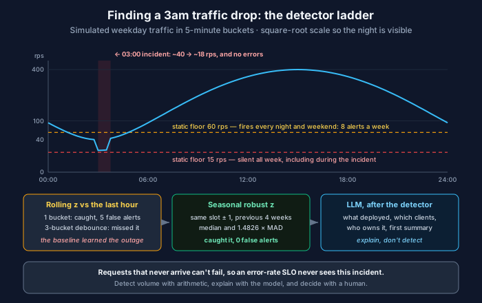
Picture an incident that pages nobody — a hypothetical, but a common shape. It’s 03:00 on a Tuesday. A mobile release has broken a background sync, and traffic to your API falls from its usual nightly 40 requests per second to about 18. No errors — the requests that stopped arriving can’t fail. Latency is fine. Every dashboard is green, and it stays green until the morning, when someone notices the afternoon peak is short by half.

This post builds a detector that catches it, one rung at a time. Each rung fixes the previous rung’s failure and has a new one of its own. Every number below comes from the script at the end, which you can run.

Rung 1: the static threshold

The first thing everyone writes: page if traffic drops below some floor.

The trouble is picking the number. This service peaks around 440 rps in the afternoon and bottoms out around 40 at night, and lower still at weekends. Over one simulated week:

• Floor at 60 rps catches the incident — and fires 8 times, because every night and every weekend trough is below 60.
• Floor at 15 rps is silent all week, including during the incident, which averaged about 18.

There is no number that works, because “normal” moves tenfold over a day. Static thresholds are fine for quantities with a fixed healthy range: disk usage, queue depth against a hard limit, days until a certificate expires. They fail for anything with a cycle, and almost all traffic has one.

Rung 2: the rolling baseline

So compare against recent history instead of a constant. Take the last hour, compute the mean and standard deviation, and alert when the current value is more than four standard deviations away. This is a z-score, and it adapts to the time of day automatically.

On a single bucket, it catches the incident — along with 5 false alerts in the week, because ordinary noise occasionally lands four deviations out.

The standard fix for noise is a debounce: only alert after three consecutive anomalous buckets. Add it, and the false alerts disappear. So does the incident.

What happened is the most important failure in this whole post. By the third bucket of the outage, the first two outage buckets are in the baseline. The mean has dropped, the deviation has grown, and the third bucket no longer looks unusual against a window that’s partly made of the incident itself. The baseline learned the outage.

Any adaptive baseline whose window is shorter than the incident will eventually call the incident normal. Make the window longer and you’re back to fighting the daily cycle. You need a baseline that doesn’t depend on the last few minutes at all.

Rung 3: the seasonal baseline

Traffic at 03:00 on a Tuesday should look like traffic at 03:00 on previous Tuesdays. So compare against those, not against the last hour.

Two choices matter here.

Use the median and MAD, not the mean and standard deviation. The median absolute deviation is the median of each point’s distance from the median. Both are robust: if one of the previous four Tuesdays had its own incident, the mean gets dragged towards it and the standard deviation inflates, but the median barely moves. Multiply the MAD by 1.4826 and it’s on the same scale as a standard deviation for normally distributed data, so “more than 4” still means roughly what you’d expect.

Use enough history. With only the same five-minute slot from four previous weeks — four numbers — the detector catches the incident and also fires 5 false alerts. The MAD of four points is itself a noisy estimate, so the threshold wobbles. Widen the history to include the adjacent slots on either side, and the detector has twelve points instead of four. It catches the incident with zero false alerts in the week.

Detector	Caught the incident	False alerts in a week
Static floor, 60 rps	Yes	8
Static floor, 15 rps	No	0
Rolling z, one bucket	Yes	5
Rolling z, three buckets	No	0
Seasonal robust z, same slot	Yes	5
Seasonal robust z, slot ± 1	Yes	0

The code

Standard library only. It simulates five weeks of traffic in five-minute buckets with a daily cycle and quieter weekends, injects the 03:00 incident into the fifth week, and scores each detector on that week.

import math
import random
from statistics import mean, median, pstdev

random.seed(7)
PER_DAY = 288                      # 5-minute buckets
PER_WEEK = 7 * PER_DAY


def expected_rps(i):
    day, slot = divmod(i % PER_WEEK, PER_DAY)
    hour = slot / 12
    daily = 0.55 + 0.45 * math.sin((hour - 9) / 24 * 2 * math.pi)  # trough ~03:00
    return 400 * daily * (0.6 if day >= 5 else 1.0)                 # quieter weekends


# Five weeks of traffic. Weeks 1-4 are history; week 5 is scored.
series = [random.gauss(expected_rps(i), 0.04 * expected_rps(i)) for i in range(5 * PER_WEEK)]

# The incident: Tuesday 03:00-03:45 of week 5, traffic falls to 45% of normal.
start = 4 * PER_WEEK + PER_DAY + 36
incident = set(range(start, start + 9))
for i in incident:
    series[i] *= 0.45


def mad(xs):
    m = median(xs)
    return median(abs(x - m) for x in xs)


def rolling_z(i, window=12):
    hist = series[i - window:i]                   # the previous hour
    sd = pstdev(hist)
    return sd > 0 and abs(series[i] - mean(hist)) / sd > 4


def seasonal_z(i, weeks=4, neighbours=0):
    hist = [series[i - w * PER_WEEK + d]          # same slot in previous weeks,
            for w in range(1, weeks + 1)          # optionally +/- adjacent slots
            for d in range(-neighbours, neighbours + 1)]
    spread = 1.4826 * mad(hist)                   # MAD scaled to approximate sigma
    return spread > 0 and abs(series[i] - median(hist)) / spread > 4


def debounce(flags, need):
    out, run = [], 0
    for f in flags:
        run = run + 1 if f else 0
        out.append(run >= need)
    return out


detectors = [
    ("static floor 60 rps",        lambda i: series[i] < 60,   3),
    ("static floor 15 rps",        lambda i: series[i] < 15,   3),
    ("rolling z, 1 bucket",        rolling_z,                  1),
    ("rolling z, 3 buckets",       rolling_z,                  3),
    ("seasonal z, same slot",      seasonal_z,                 3),
    ("seasonal z, slot +/- 1",     lambda i: seasonal_z(i, neighbours=1), 3),
]

scored = range(4 * PER_WEEK, 5 * PER_WEEK)
print(f"{'detector':<26}{'caught it':<11}{'false alerts this week'}")
for name, fn, need in detectors:
    fired = {i for i, a in zip(scored, debounce([fn(i) for i in scored], need)) if a}
    false = sorted(fired - incident)
    episodes = sum(1 for k, i in enumerate(false) if k == 0 or i != false[k - 1] + 1)
    print(f"{name:<26}{str(bool(fired & incident)):<11}{episodes}")

Output:

detector                  caught it  false alerts this week
static floor 60 rps       True       8
static floor 15 rps       False      0
rolling z, 1 bucket       True       5
rolling z, 3 buckets      False      0
seasonal z, same slot     True       5
seasonal z, slot +/- 1    True       0

Be honest about what this proves. The noise is Gaussian, and real traffic has heavier tails. There are no holidays, which break week-over-week comparisons badly — the Monday after a long weekend looks like an outage to a seasonal detector. There are no launches or marketing pushes, which create legitimate step changes. A production detector needs a calendar of known events and a way to suppress or rebaseline around them. The ranking of the rungs holds up; the exact counts are a property of this synthetic week.

The same idea in PromQL

You don’t need a separate system to get most of this. A week-over-week ratio against the average of the previous three weeks:

sum(rate(http_requests_total{job="api"}[5m]))
/
(
  (
      sum(rate(http_requests_total{job="api"}[5m] offset 1w))
    + sum(rate(http_requests_total{job="api"}[5m] offset 2w))
    + sum(rate(http_requests_total{job="api"}[5m] offset 3w))
  ) / 3
)
< 0.6

Put it in an alerting rule with for: 15m as the debounce. It’s a mean rather than a median, so one bad week in the history skews it — the trade you make for a one-line rule. If you’ve used Prometheus’s built-in smoothing function, note that in Prometheus 3 holt_winters was renamed double_exponential_smoothing and now needs --enable-feature=promql-experimental-functions. Rules that used the old name stop working after the upgrade.

When not to use anomaly detection

For user-facing errors and latency, don’t page on anomalies. Page on your SLO burning. The SRE Workbook’s multiwindow, multi-burn-rate recommendation for a 99.9% SLO:

Severity	Budget consumed	Long window	Short window	Burn rate
Page	2%	1 hour	5 minutes	14.4
Page	5%	6 hours	30 minutes	6
Ticket	10%	3 days	6 hours	1

The short window is there for the same reason as the debounce problem above, in reverse: it lets the alert stop firing soon after the errors stop, instead of waiting for the long window to drain.

Burn-rate alerts are better pagers because they’re tied to an objective users actually feel, and their thresholds come from arithmetic on a budget rather than from staring at a graph. Anomaly detection earns its place on the things an SLO can’t see. The opening incident is the canonical one: traffic that stops arriving produces no errors. An error-rate SLO is a ratio of failed requests to received requests, and requests that were never sent are in neither number. You need a detector on the volume itself.

Where the LLM belongs

It’s tempting to hand the whole problem to a model: give it the graph, ask if anything looks wrong. The research says that’s the wrong division of labour. The SigLLM study (Alnegheimish et al., MIT, 2024) found LLMs can detect time-series anomalies zero-shot — and that state-of-the-art deep learning detectors still did about 30% better across eleven datasets. Using the model as a forecaster beat prompting it to point at anomalies directly, which tells you something: the model did best when it was used as a statistical component.

Then there’s cost. A detector on every series at every five-minute interval is millions of evaluations a day. The median and MAD are free. A model call isn’t.

So here’s the split I’d use:

• Detect with arithmetic. It’s cheap, deterministic, explainable in one sentence (“traffic is 4.8 MADs below the same hour over the last four weeks”), and it doesn’t hallucinate.
• Explain with the model. Once the detector fires, an LLM is very good at the next twenty minutes of work: what deployed recently, which clients’ traffic dropped, whether the drop lines up with a release, which team owns the thing, and a first-draft summary. That’s where AI triage actually pays.
• Decide with a human, at least until the agent has earned the autonomy.

The anomaly at 03:00 doesn’t need intelligence to find. It needs the right baseline. The intelligence is for the part after: working out why.

---

Related: SLI, SLO, SLA, and error budgets · Percentiles, Properly: You Cannot Average a p99 · Alert fatigue? Let AI triage.