Aug 2, 2026 · 8 min read AI Platform Engineering FinOps

GPU utilization is a lying metric: the unit economics of self-hosted inference

You can run a GPU at 100% utilization and waste most of it. The cost model that predicts your inference bill, and the five levers in payback order.

Diagram: two LLM inference servers with the same GPU utilization but different useful token throughput, followed by the five payback-ordered cost levers

Here’s a thing that took me longer to internalize than it should have.

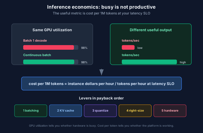
You can run an A100 at 98% utilization and be wasting most of it.

Not in a subtle way. In a “you are paying ten times what you need to” way. The GPU is genuinely busy. The metric is not lying about the hardware state — it’s lying about what you care about, which is tokens out the door per dollar. And because utilization is the number that appears on every dashboard and every FinOps review, a lot of teams have optimized their way into a corner using a metric that can’t see the problem.

I want to lay out the cost model that does work, the levers in the order they actually pay, and a break-even calculation for the self-host-vs-API question that most people are answering with vibes.

One scoping note: this is about serving models on GPUs you rent or own. If you buy tokens from a hosted API, your cost problems are real but different — that’s token FinOps, and it’s a metering and attribution discipline. This post is about the unit economics underneath the token.

Why utilization can’t see it

LLM inference has two phases with completely different hardware characteristics, and conflating them is the root of most bad cost intuition.

Prefill processes your prompt. It’s compute-bound — it saturates tensor cores and scales with prompt length. It’s the phase that behaves the way you expect a GPU to behave.

Decode generates tokens one at a time. Each token requires reading the entire model’s weights from high-bandwidth memory to produce a single token. It is memory-bandwidth-bound, and at batch size 1 the tensor cores are largely idle, waiting.

That’s the trap. A decode-heavy server at batch size 1 shows high utilization because the memory subsystem is pinned. Push it to batch size 32 and each weight read now serves 32 sequences instead of one. Utilization barely moves. Throughput goes up roughly an order of magnitude.

Utilization measures busy. You’re paying for productive. For inference those diverge violently, and the divergence is the whole opportunity.

The metric that works:

cost per 1M tokens = (instance $/hour ÷ tokens/hour at your latency SLO) × 1,000,000

The “at your latency SLO” clause is load-bearing. Throughput and latency trade against each other — larger batches raise throughput and raise time-to-first-token. A cost-per-token number without a latency constraint attached is a number you can improve indefinitely by making the product unusable.

Measure it like this, not from a spec sheet:

# Output tokens per second, actually served
sum(rate(vllm:generation_tokens_total[5m]))

# Prefill tokens per second — usually the ignored half of your bill
sum(rate(vllm:prompt_tokens_total[5m]))

# Are you actually batching? If this hovers near 1, stop reading and go fix it.
avg(vllm:num_requests_running)

# The constraint your cost number must respect
histogram_quantile(0.95, sum(rate(vllm:time_to_first_token_seconds_bucket[5m])) by (le))

If num_requests_running sits near 1 under real load, nothing else in this post matters yet. That’s the finding.

The five levers, in payback order

I’ve seen this list attempted in almost exactly reverse order — buy more GPUs first, quantize in a panic later — so the ordering is the actual advice.

1. Continuous batching (config change, 3–4x)

Naive batching gathers a fixed group, runs it, and waits for the slowest sequence before starting the next group. Since request lengths vary enormously, short requests sit finished-but-blocked while one long generation drags on.

Continuous batching works at the iteration level: the moment any sequence completes, its slot is refilled from the queue. No batch boundaries, no waiting for stragglers. The reported delta is typically 3–4x throughput on identical hardware.

Every serious stack supports it — vLLM, SGLang, TensorRT-LLM. Which means the teams not getting this are the teams who deployed with defaults from a tutorial and never revisited it. Check first. It is the cheapest 3x you will ever find.

2. KV cache and prefix reuse (the big one for agents)

Paged attention ships by default in every 2026 production stack, so you probably have the mechanism. The question is whether your architecture lets you use it.

A cache hit on a shared prefix means prefill compute that never happens — the self-hosted analogue of prompt caching, except you own the eviction policy and therefore the eviction problem. Published engineering analyses put combined KV cache techniques at 4–40x cost reduction for long-context inference, and the upper end of that range is specifically workloads with heavy prefix sharing.

Which is to say: agent workloads. An agent loop resends a growing transcript on every single step. Step 12 shares its entire prefix with step 11. If your prompt is constructed so the stable content sits at the front and the variable content at the back, nearly all of that prefill is free. If you interpolate a timestamp or a request ID near the top of your system prompt, you have invalidated the cache for every request in your fleet, forever, and your bill reflects it.

I’ve seen exactly that bug twice. Both times it was one line. Both times it was worth a meaningful fraction of the inference budget.

The other half is routing: a cache hit only helps if the request lands on the replica holding the cache, which is a load balancing problem, not a serving problem. That’s what the Inference Gateway exists to fix, and it’s why cache-aware routing improves latency and cost simultaneously — a rare combination.

Also worth reading with this: context engineering. Cache economics and context discipline are the same subject approached from different ends.

3. Quantization (1.3–2x, mild quality cost)

FP8 on H100-class hardware, natively supported in vLLM, commonly gives 1.3–2x throughput over FP16 at under 2% quality degradation on instruction-tuned models. INT4 and other aggressive schemes go further with correspondingly more risk.

The reason this is third rather than first isn’t that it’s small — it’s that it’s the first lever with a quality cost, and therefore the first one that needs an evaluation harness before you turn it on. Deploy an eval set for your actual task, measure before and after, and treat “under 2%” as a claim to verify on your workload rather than a guarantee. Without that harness you’re not optimizing, you’re gambling with a metric nobody is watching.

4. Right-size the model to the task

This is a bigger topic than a bullet — see the SLM tier — but in cost terms the summary is blunt: serving a 7B model is roughly an order of magnitude cheaper than a 70B+ model, and a large share of production traffic is classification, extraction, routing, and formatting, where the larger model’s advantage is invisible.

Auditing which requests actually need your biggest model is usually the highest-value hour anyone spends on inference cost, and it requires no infrastructure change at all.

5. Infrastructure: fractional GPUs and spot

Now, and only now, touch the hardware layer.

Fractional GPUs — MIG, time-slicing, MPS — matter when you serve small models that can’t fill a card. An A100 running a 3B model at low traffic is mostly billed idle capacity. MIG partitions turn one card into several isolated ones. This is the closest thing inference has to bin-packing, and most clusters aren’t doing it.

Spot capacity for anything interruptible: batch scoring, embedding generation, evals, offline classification. Not for latency-sensitive serving unless you’ve built genuinely robust drain-and-migrate, and be honest about whether you have.

More replicas is the last resort, not the first. Adding a replica to a fleet running at batch size 2 buys you more expensive idle capacity.

The break-even question

“Should we self-host or use an API?” is asked as a rate comparison and is actually a utilization question. A dedicated GPU bills 24 hours a day. An API bills per token. So self-hosting wins above a volume threshold and loses — often catastrophically — below it.

Here’s the calculator. It includes the two inputs people leave out, which are the two that usually decide it:

#!/usr/bin/env python3
"""Break-even analysis: self-hosted inference vs hosted API.

The defaults below are illustrative. Replace every one of them with
numbers measured on your own workload — especially tokens_per_second,
which must be measured at your latency SLO, not from a benchmark blog.
"""

from dataclasses import dataclass


@dataclass
class SelfHosted:
    instance_cost_per_hour: float      # on-demand or committed rate
    replicas: int
    tokens_per_second: float           # MEASURED, at your p95 TTFT target
    duty_cycle: float                  # fraction of hours actually serving load
    engineer_fte: float                # fraction of an FTE operating this
    engineer_cost_per_year: float

    def monthly_cost(self) -> float:
        hours = 730
        infra = self.instance_cost_per_hour * self.replicas * hours
        people = (self.engineer_fte * self.engineer_cost_per_year) / 12
        return infra + people

    def monthly_tokens(self) -> float:
        seconds = 730 * 3600 * self.duty_cycle
        return self.tokens_per_second * self.replicas * seconds

    def cost_per_million(self) -> float:
        tokens = self.monthly_tokens()
        return (self.monthly_cost() / tokens) * 1_000_000 if tokens else float("inf")


@dataclass
class HostedAPI:
    input_cost_per_million: float
    output_cost_per_million: float
    input_output_ratio: float = 4.0    # typical: prompts dwarf completions

    def cost_per_million(self) -> float:
        r = self.input_output_ratio
        return (self.input_cost_per_million * r + self.output_cost_per_million) / (r + 1)


def breakeven_tokens_per_month(sh: SelfHosted, api: HostedAPI) -> float:
    """Monthly token volume above which self-hosting is cheaper."""
    api_rate = api.cost_per_million() / 1_000_000
    return sh.monthly_cost() / api_rate if api_rate else float("inf")


if __name__ == "__main__":
    # ILLUSTRATIVE INPUTS — substitute your own
    sh = SelfHosted(
        instance_cost_per_hour=3.50,
        replicas=2,
        tokens_per_second=850,        # measured at p95 TTFT < 800ms
        duty_cycle=0.35,              # be honest: nights and weekends count
        engineer_fte=0.25,
        engineer_cost_per_year=220_000,
    )
    api = HostedAPI(input_cost_per_million=3.00, output_cost_per_million=15.00)

    print(f"Self-hosted monthly cost:   ${sh.monthly_cost():>12,.0f}")
    print(f"Self-hosted monthly tokens: {sh.monthly_tokens():>13,.0f}")
    print(f"Self-hosted $/1M tokens:    ${sh.cost_per_million():>12,.2f}")
    print(f"API blended $/1M tokens:    ${api.cost_per_million():>12,.2f}")
    print(f"Break-even volume/month:    {breakeven_tokens_per_month(sh, api):>13,.0f} tokens")

    verdict = "self-host" if sh.cost_per_million() < api.cost_per_million() else "API"
    print(f"\nAt current volume and duty cycle: {verdict}")
    print("Now re-run with duty_cycle=0.10 and see what happens.")

Run it with duty_cycle=0.10. That’s the experiment that matters, and it’s the number nobody puts in the business case. A cluster sized for peak and idle overnight is billing you at full rate for every idle hour. I have watched self-hosting decisions justified on peak-hour arithmetic and then quietly lose money for a year, because the model in the spreadsheet assumed a duty cycle nobody ever checked.

The engineer_fte input is the other one. Operating a serving stack is not free — someone patches vLLM, chases OOMs, manages driver upgrades, and gets paged. A quarter FTE is not a pessimistic estimate for a real production deployment; it’s often generous.

None of which means don’t self-host. Self-hosting wins on sustained high volume, data residency, latency floors, and model control, and those are frequently the actual reasons — which is fine, as long as the cost argument isn’t being used to launder a decision made for other reasons. Say the real reason out loud. It’s usually a better argument anyway.

What I’d actually do this quarter

If you inherited an inference platform tomorrow, in order:

Graph avg(num_requests_running) under peak load. If it’s near 1, fix batching. Stop here until it’s fixed.
Compute your real cost per million tokens at your p95 latency target. Not utilization. Not $/GPU-hour.
Audit prompt construction for cache-invalidating content near the front. Look for timestamps, UUIDs, and user names in system prompts.
Count what fraction of requests genuinely need your largest model.
Compute duty cycle honestly, then re-run the break-even.

That’s a week of work and it routinely finds several multiples. Meanwhile the thing most orgs do first — negotiating GPU pricing — moves the number by maybe 20%.

The deeper point is one that generalizes past inference. AI infrastructure is new enough that we’re still using metrics inherited from the last era of infrastructure, and some of them measure the wrong thing now. Utilization was a good proxy when work was compute-bound and roughly uniform. Inference is neither. The dashboards haven’t caught up, and the money is sitting in the gap.

Sources: KV Cache Optimization for LLMs 2026: Engineering Guide · AI Inference Cost Optimization: FinOps Playbook 2026 · Kubernetes GPU Cost Crisis · Cutting LLM Inference Costs in 2026 (GMI Cloud)

Frequently asked questions

Why is GPU utilization a bad metric for LLM inference cost?

Because utilization measures whether the GPU is busy, not whether it is producing useful output. An LLM server decoding one request at batch size 1 can report near-100% utilization while the tensor cores sit mostly idle waiting on memory bandwidth — decode is memory-bound, not compute-bound. The same GPU running continuous batching at batch size 32 reports the same utilization number and serves an order of magnitude more tokens. The metric that predicts your bill is cost per million tokens served at your latency SLO, which requires throughput, price, and the latency constraint in the same equation.

What are the highest-impact levers for reducing LLM inference cost?

Five, roughly in payback order. First, continuous batching — moving from naive to continuous batching is typically a 3–4x throughput gain on identical hardware, and it is a configuration change. Second, KV cache management and prefix reuse, which for long-context and multi-turn workloads is the single largest lever available. Third, quantization — FP8 on H100-class hardware via vLLM commonly yields 1.3–2x throughput over FP16 at under 2% quality loss on instruction-tuned models. Fourth, right-sizing the model to the task rather than routing everything to the largest one. Fifth, infrastructure levers: fractional GPUs via MIG or time-slicing for small models, and spot capacity for interruptible batch work. Adding replicas is last, not first.

When does self-hosting inference become cheaper than a hosted API?

It is a utilization question, not a rate question. A dedicated GPU bills whether or not you use it, so self-hosting wins above a break-even token volume and loses badly below it. Compute your effective cost per million tokens as (hourly instance cost ÷ tokens served per hour at your latency SLO), then compare to the API's blended input/output rate. Two factors dominate the result and are routinely omitted: the engineering cost of operating the stack, and your actual duty cycle — a cluster sized for peak and idle at 3am is billing you for the idle hours at full rate. Bursty low-volume workloads almost always lose.

What is continuous batching and why does it matter so much?

Naive batching collects a fixed group of requests, runs them together, and waits for the slowest to finish before starting the next group — so short requests sit idle waiting on long ones. Continuous batching operates at the iteration level: as soon as any sequence in the batch completes, its slot is refilled with a waiting request. The GPU never waits for a batch boundary. Because inference request lengths vary enormously, this recovers a large share of otherwise-wasted capacity, typically 3–4x throughput on the same hardware. Every major serving stack — vLLM, SGLang, TensorRT-LLM — supports it, which means many teams paying for it are not enabling it.

Does KV cache optimization actually reduce cost or just latency?

Both, and that makes it unusual. Most latency optimizations cost money and most cost optimizations cost latency. Prefix caching removes prefill compute you would otherwise pay for — a cache hit on a shared system prompt or conversation history is arithmetic that simply does not happen. Published engineering analyses put combined KV cache techniques at 4–40x cost reduction for long-context inference, with the top of that range applying to workloads with heavy prefix sharing such as agent loops that resend a growing transcript on every step.