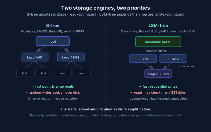
The same job — persist key-value data on disk — solved with opposite priorities.
Pick any database and ask one question: is its storage engine a B-tree or an LSM-tree? Almost everything else about how it behaves under load follows from the answer. Postgres, MySQL’s InnoDB, and most traditional relational databases are B-trees. Cassandra, RocksDB, ScyllaDB, and the storage layer under a lot of modern vector databases are LSM-trees. This is a refresher on why that one architectural choice ripples through everything you feel in production.
The problem both are solving
Disks — even SSDs — have a personality. Sequential writes are cheap; random writes are expensive. A storage engine’s entire job is to keep your data sorted and findable on disk while working with that personality instead of against it. B-trees and LSM-trees make opposite bets about how to do it.
B-trees: update in place, optimize for reads
A B-tree keeps data sorted in a shallow, wide tree of fixed-size pages, as on the left of the diagram. Every lookup starts at the root and walks down a handful of levels to the leaf — O(log n), and because the tree is wide, that’s typically only 3–4 disk pages even for billions of rows. Range scans are excellent because the leaves are kept in sorted order.
The price is on writes. To update a row, the engine finds its page and mutates it in place. When rows scatter across the key space, those writes scatter across the disk — random I/O, the expensive kind. The B-tree also maintains a write-ahead log for durability, so a single logical write can touch the log and the page. This is fine for many workloads and genuinely bad for write-heavy ones like high-volume event ingestion.
B-trees win when: reads dominate, you need range queries and strong ordering, and your write rate is moderate. That describes most transactional business applications, which is why the relational default is a B-tree.
LSM-trees: never overwrite, optimize for writes
An LSM-tree (Log-Structured Merge-tree) refuses to do random writes at all. New writes go into an in-memory sorted structure — the memtable (right side of the diagram). When it fills, it is flushed to disk as an immutable, sorted file: an SSTable. That flush is one big sequential write. You never go back and edit an SSTable; you just keep making new ones.
This makes writes blazing fast, but it pushes the cost onto reads and onto housekeeping:
- Reads may have to check several SSTables — the newest first, falling back to older ones — because a key’s latest value could live in any of them. Engines soften this with in-memory indexes and, crucially, Bloom filters that let a read skip an SSTable it definitely isn’t in.
- Compaction runs in the background, merging SSTables, discarding overwritten and deleted keys, and keeping read amplification bounded. Compaction is the LSM-tree’s defining operational characteristic: it is where your disk bandwidth and CPU quietly go, and a mistuned compaction strategy is behind a large share of “the database is fast except when it randomly isn’t” incidents.
LSM-trees win when: writes are heavy and continuous — time-series, event logs, metrics, IoT ingest — and you can tolerate reads doing a bit more work.
The two words that summarize the trade
- Read amplification — one logical read causing several physical reads. LSM-trees have more of it.
- Write amplification — one logical write causing several physical writes (the memtable flush, then every compaction that later rewrites that data). LSM-trees also have more of this, which matters for SSD wear.
There is no free lunch. You are choosing which amplification you would rather pay, based on your workload’s read/write mix. That is the whole decision.
Why this matters in the AI/cloud era
This is not a legacy topic. It has quietly moved to the center of AI infrastructure.
Vector databases are storage engines too. The approximate-nearest-neighbor index gets the attention, but underneath it there is still a key-value engine storing vectors, IDs, and metadata — and its choice of B-tree vs LSM shapes ingest throughput and query latency. AI pipelines that stream embeddings in continuously (re-indexing a knowledge base as documents change) are write-heavy workloads, and that pushes toward LSM-style engines. If your RAG ingestion is fast but your retrieval tail latency is ugly, read amplification and compaction pressure are prime suspects.
Feature stores and telemetry are write-firehoses. The observability data behind AI systems — every token, every tool call, every latency sample — is exactly the append-heavy, time-ordered workload LSM-trees were built for. It is not a coincidence that the databases underneath modern metrics and tracing stacks are LSM-based.
Managed cloud databases hide the engine but not its behavior. DynamoDB, Bigtable, and Cassandra-as-a-service abstract the storage engine away, right up until you hit a performance cliff. Knowing whether you are sitting on a B-tree or an LSM-tree tells you which cliff — a slow-range-scan cliff or a compaction-stall cliff — and that turns a mystifying latency graph into a solvable problem.
The takeaway
You do not need to implement either one. You need to be able to ask, of any database you adopt: which engine is this, and does its bet match my workload’s read/write balance? Get that match right and the database feels effortless. Get it wrong — a write-firehose on a B-tree, or a range-scan-heavy analytics job on an LSM-tree — and you will spend months fighting the storage layer while blaming everything above it. The two boxes in the diagram are, more than any config flag, the thing that decides how your data layer behaves.
Comments