You change a prompt. Your eval suite goes from 80% to 84%. You ship it.
Here’s how often that happens when the new prompt is exactly as good as the old one, simulated 20,000 times per eval size:
| Cases in the eval | Identical prompts look 3+ points better | Look 5+ points different either way |
|---|---|---|
| 20 | 40.3% | 66.8% |
| 50 | 31.9% | 44.5% |
| 100 | 26.9% | 28.1% |
| 200 | 18.3% | 12.2% |
| 500 | 7.4% | 1.4% |
| 1,000 | 2.0% | 0.05% |
On a 50-case eval, a coin-flip-level improvement shows up about one time in three. I’ve written before about what a single score on a small set can and can’t tell you. This post is about the next question: comparing two runs, which is what you’re doing every time you touch a prompt.
The setup
In the simulation, every eval case has its own pass probability, drawn from a Beta distribution with a mean of 80%. Some cases almost always pass, some almost never do, and a few are genuinely flaky. Two runs over the same cases are correlated, as they are in real life. All of it is seeded and in the repo.
Use the pairing you already have
Both versions ran on the same cases, so the useful data is the flips:
| B passes | B fails | |
|---|---|---|
| A passes | both pass | lost |
| A fails | gained | both fail |
Cases where both versions agree tell you nothing about which is better. Only gained and lost matter. If the versions were equal, each flip would be a fair coin, so you can test it with a binomial. That’s McNemar’s test from 1947, and the exact version is three lines:
def mcnemar_exact(b, c):
    n = b + c
    if n == 0:
        return 1.0
    return min(1.0, 2 * sum(comb(n, i) for i in range(min(b, c) + 1)) / 2**n)
Run on identical prompts, it fired 2.2% of the time at 50 cases and 4.3% at 1,000, below its nominal 5% because the exact test is conservative. Compare that with the 32% from eyeballing the difference.
A real improvement is harder to see than you think
Now give B a true 3-point improvement and ask how often the test notices:
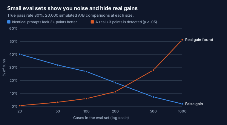
At 100 cases, a real 3-point gain is detected 6% of the time. At 1,000, 51%. On any eval set you are likely to have, a 3-point improvement is invisible, and identical prompts produce fake 3-point improvements more often than the test finds real ones.
To plan the size, use Connor’s formula for paired designs. For small effects it reduces to something you can do in your head:
n ≈ 7.85 × D / d², where D is the share of cases where the two versions disagree, and d is the effect you want to detect.
| Effect to detect | Disagree on 10% | Disagree on 20% | Disagree on 40% |
|---|---|---|---|
| +1 point | 7,847 | 15,696 | 31,394 |
| +2 points | 1,960 | 3,923 | 7,847 |
| +3 points | 870 | 1,742 | 3,487 |
| +5 points | 312 | 626 | 1,254 |
| +10 points | 77 | 155 | 312 |
Those are the cases needed for 80% power at p < 0.05. Read that table before you promise anyone a 2-point improvement.
Reducing disagreement is the cheapest way to shrink the table. Halving D halves n. Deterministic graders, frozen tool responses and fixing your flakiest cases all pay off directly here.
When pairing helps, and when it doesn’t
I expected paired tests to win everywhere. They don’t. The advantage depends on how stable each case’s outcome is:
| Power at n = 1,000, true +3 points | Paired (McNemar) | Unpaired z-test |
|---|---|---|
| Stable cases (mostly always-pass or always-fail) | 76.0% | 35.4% |
| Mixed | 51.3% | 39.2% |
| Every case equally flaky | 39.9% | 40.4% |
When outcomes are stable, the pairing cancels the case-to-case variation and doubles your power. When every case is a coin flip of the same bias, there’s nothing to cancel and the two tests tie. Pairing costs nothing, so use it regardless, but if your agent is flaky on every case, a better test won’t save you.
The winner’s curse
The worst version of this is the prompt optimizer, whether it’s a tool or an engineer on a long afternoon. Try 20 variants, keep the best. I simulated that with 20 variants that were all truly identical to the baseline:
| Cases | Apparent gain of the winner | True gain | Passes p < .05 uncorrected | Passes after Bonferroni |
|---|---|---|---|---|
| 50 | +8.1 points | 0 | 10.1% | 0.4% |
| 100 | +5.9 points | 0 | 14.2% | 1.1% |
| 200 | +4.2 points | 0 | 16.0% | 1.4% |
| 500 | +2.7 points | 0 | 17.1% | 1.5% |
Selection manufactures an improvement from nothing. A dev set you’ve optimized against is no longer evidence, which is why anything that picks among candidates needs a holdout it never touched, and why the multiple-comparison correction (divide your p-value threshold by the number of candidates) is not pedantry.
What I’d do with this
Report flips, not scores. “Gained 9, lost 3, here are the IDs” is more useful in a PR than “84%”, and someone can actually read the three.
Gate CI on regressions only. Block a change that is significantly worse. Don’t block one that fails to prove it’s better, because at realistic eval sizes almost nothing can.
Decide the effect size before you run. If only a 10-point change would alter your decision, 155 cases are enough. If you’re hunting 1-point gains, you need a production A/B test, because an offline eval won’t get there.
Keep a holdout you only look at once per decision.
The tool is one stdlib-only file:
python eval_compare.py baseline.jsonl candidate.jsonl --fail-on-regressioncases 200
baseline 80.0%
candidate 83.5%
difference +3.5% (95% CI -2.3% to +9.3%)
flips +21 gained, -14 lost
McNemar exact p 0.3105
verdict no_detectable_differenceThe interval is Agresti and Min’s for matched proportions. That’s the tool’s real output on a made-up pair of runs, and it’s the common case: a score that went up and a verdict that says you don’t know yet.
Limits
This is a model of eval behaviour, not data from a specific system. It assumes binary pass or fail, independent cases and perfect grading. A noisy LLM judge adds disagreement that pushes every number in the sample-size table up. Correlated cases (ten variants of one scenario) make your real n smaller than your row count.
Code, tests and every result: ajinb/eval-compare.
Comments