Big-O Notation in the Age of Billion-Vector Search

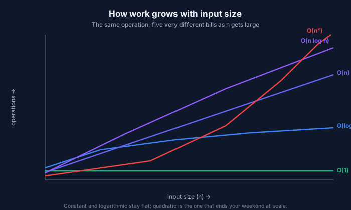
How the same operation bills you very differently as the input grows.

Big-O notation is the first thing taught in an algorithms course and the first thing forgotten once the framework does the heavy lifting for you. Then one day a service that was fast in staging falls over the moment real traffic arrives, and it turns out the answer was on a whiteboard the whole time. This is a refresher on the one piece of theory that has never stopped being load-bearing — and why it matters more, not less, in a world of vector databases and million-token context windows.

What Big-O actually measures

Big-O describes how the work an algorithm does grows as its input grows. It is deliberately not a stopwatch. It throws away constant factors and lower-order terms so you can compare the shape of two algorithms without caring about the language, the CPU, or the year.

The shapes you meet most often, from best to worst:

• O(1) — constant. The work does not change with input size. A hash-map lookup. Reading an array by index.
• O(log n) — logarithmic. Each step throws away half the remaining work. Binary search. A balanced-tree lookup.
• O(n) — linear. You touch every element once. Scanning a list.
• O(n log n) — linearithmic. The practical floor for comparison sorting. Merge sort, quicksort on average.
• O(n²) — quadratic. A loop inside a loop over the same data. Fine at n=100, a catastrophe at n=1,000,000.

The chart above is the whole intuition. At small n the curves are indistinguishable — which is exactly why the quadratic bug ships. It is only when n gets large that O(n²) peels away from the pack and turns a 200ms request into a 40-second one.

Why constants still lie to you

Big-O ignores constant factors, and in interviews that is correct. In production it is a trap. An O(n) algorithm with a huge constant — say, a network round-trip per element — can be slower than an O(n log n) algorithm that stays in cache, right up until n gets big. The mental model is: Big-O tells you which algorithm wins eventually; the constant tells you where “eventually” starts. You need both. A cache-friendly O(n²) can beat a pointer-chasing O(n log n) for the first few thousand elements, which is why real sort implementations switch to insertion sort for small partitions.

The AI-era version of the same mistake

You would think a topic this old would have nothing to say about modern AI infrastructure. It has everything to say about it.

Vector search is a complexity problem wearing a new hat. A naive similarity search compares your query vector against every stored vector — that is O(n) per query, and with a billion vectors and a metric like cosine similarity over 1,536 dimensions, the constant is enormous. This is the entire reason approximate-nearest-neighbor indexes (HNSW, IVF) exist. They trade exactness for complexity, turning an O(n) scan into something closer to O(log n) by building a graph or an inverted index up front. When someone asks “why is our RAG retrieval slow,” the honest answer is usually “you are doing a linear scan and calling it a vector database.”

The attention mechanism is O(n²) in sequence length. Every token attends to every other token, so doubling the context window quadruples the compute for that step. That single fact explains most of the last few years of ML systems research — flash attention, sliding windows, sparse attention — all of it is an attempt to beat a quadratic curve. When a vendor announces a longer context window, they are announcing that they found a way to bend that O(n²).

Prompt and token growth are linear costs you pay per request, forever. Stuffing more context into every call is O(n) in tokens, and unlike a one-time index build, you pay it on every single request. The context window is a budget, and Big-O is the accounting.

How to use it without a chalkboard

You do not need to derive complexity from first principles to get the benefit. Three habits cover most of it:

1. Find the nested loop. The most common accidental O(n²) is a loop that, inside it, does a linear search or a database query per iteration. Turn the inner lookup into a hash map and you often drop straight to O(n). This one pattern is responsible for a disproportionate share of “it got slow as we grew” incidents.
2. Ask what happens at 100×. Not double — 100×. Linear and logarithmic algorithms shrug. Quadratic ones fall over. If the answer is “we’d need 100× the machines,” you have found a complexity problem, not a capacity problem.
3. Know the complexity of the thing you are calling. x in a_list is O(n). x in a_set is O(1). list.insert(0, x) is O(n). Most performance bugs are not exotic — they are the wrong container.

Why this endures

Frameworks change, languages come and go, and the accelerator in the rack is different every eighteen months. But the relationship between input size and work is a property of the algorithm, not the hardware — and no amount of faster silicon changes an O(n²) into an O(n log n). That is why Big-O has outlasted every technology it was ever taught alongside, and why it will quietly decide whether your next AI-native system scales or stalls. The demo runs on small n. Production does not.